Tuesday, September 10, 2013

Visualizing panel curvature


The Buildz blog has an excellent post on tools for checking the curvature of panels in a curved surface . However, I thought there might be an easier way. I found a method that uses Filters in Visibility graphics and shared reporting parameters. It is easy to understand and in some ways better. It does not require a special panel family for reporting the curvature. Instead, it works with any panel that has curvature.

A panel

To illustrate, start by creating a new curtain panel pattern based family. Use a Rectangular pattern. Pull the adaptive points out of the default plane. Draw reference lines for the diagonals. Place a point on each diagonal reference line. Move each point to the midpoint by setting its Normalized Curve Parameter to 0.5.


Draw a reference line between the two diagonal midpoints. This will be the measurement for how far out of a plane the panel is.

Set the Workplane to be this measuring line. Add a dimension between the two midpoints on this workplane.


Make the dimension into a parameter by using the Label tool. Make it an Instance parameter and a reporting parameter. Make it a shared parameter and call it outOfPlane.


Use Create Form to make a surface that connects all of the four adaptive points.


That’s the panel. Adding a measurement like this can be done to any panel. The color will be handled by Visibility Graphics of the view using Filters.

A curved surface

The next step is to make a curved surface. You can load one that you have already created or make a new one.

To make a new one, create a new Conceptual Mass. I made some reference planes to control the profiles of a curved surface. I drew four curves, one on each reference plane. Activate each reference plane to draw a reference line using Spline Through Points.


Use the Create Form tool to convert this into a surface.


Dividing the surface

Load the panel into the conceptual mass. Choose the conceptual mass object to select it.  Click Divide Surface to make a divided surface. Use the Type Selector to set your panel to be the type.

The conceptual model has all of the information about curvature of each panel. Once we have inserted it into a Project file, we can now use the Schedules and Visibility/Graphics with filters to inspect the curvature.

Create a new Project. Load the conceptual mass defining the surface into the new project.

To inspect the out of plane value for each panel, create a new schedule. (You may have to make sure that the shared parameter file is loaded.)


To obtain a color-coded visualization, select a view, such as the 3D view. Open the Visibility Graphics dialog, and choose the Filters tab. Create a New filter, and give it an appropriate name.


Check the Curtain Panel for the Categories. In the Filter Rules, pull down the Filter by: drop down menu and choose More parameters ….


Use the Add parameter button to reach the Parameter Properties dialog. Set the new parameter to be a shared parameter and choose your parameter for measuring flatness. Apply the parameter to Curtain Panels and close the dialog.


In the filter Rules section of the Filters dialog, select the outOfPlane parameter. Choose the criteria to be “is less that or equal to” and set the value to be 2”.
Copy this filter a couple of times and set additional filter rules criteria.


In the Visibility / Graphics dialog, add your new filters.

Change the Projection Surface Patterns for each filter to be a different color.


My surface is acceptable. I can change the filters to get a more detailed analysis of the surface. I can change the surface to increase the curvature or decrease the curvature.

A more dramatically curved surface shows some overly curved panels.


Summary

This method uses a reporting parameter of the panel to retrieve the amount that the panel is out of perfect flatness. This parameter is used by filters in Visibility/Graphics to colorize the surface. It can also be used to create a schedule of all of the panels.

In comparison to the method on the buildz blog, this method is very simple and straightforward, requiring no helper objects or duplicate panels. Also, this method can be applied to any panel being designed as a simple reporting parameter. The color coding is done in the project that uses the panel. For greater variation of the color coding, one need only add more filters. The filters only affect one view. Other views may still provide a realistic coloration of the surface. However, one can apply filters in other views by using a template. 

Thursday, September 5, 2013

Mathematically derived surfaces in Revit

Introduction

Curved surfaces have been a theme of contemporary architecture for the last twenty years.

Mathematically, a curve is the result of sweeping a line through space. A line is the result of translating a point through space. Curvature is the result of the line being swept in a formula that defines a changing vector of movement.

From the engineering and construction standpoint, there are many interesting curves, such as sine wave, hyperbolic paraboloids, and conic sections. A catenary is particularly interesting because it describes the drape of a cable or chain between two points when the load is equal along the chain. It describes the form of tension structures such as a suspension bridge or the Munich Olympic Stadium by Frei Otto. Flipped over, a catenary arch is a very efficient form for compression structures, as exploited by Gaudi in the design of the Sagrada Famigilia in Barcelona. The ability to design mathematically determined surfaces is clearly a worthwhile skill.

A Point with Formulas

From the mathematical standpoint, the surface begins with a formula for a point along a line. In Revit, the first step is to create a point that can vary in height based on an input value. Open the family template for a conceptual mass. Use the Reference Point tool to add a point at the intersection of the reference planes, assuring that you use Draw on Workplane.

This first point will be our insertion point on a flat plane that defines the x and y location of the point on the surface. Name this point Location.

If you click on this point, you will see an icon for a coordinate system. Every point is placed on a workplane that defines a coordinate system and defines additional coordinate systems. By clicking the Mirrored and Flipped property check boxes, you can change the orientation of the coordinate system. By putting in a Rotation angle, you can also change the coordinate system. When you press the space bar, you toggle between a “world” coordinate system and a “local coordinate system. Before proceeding, make sure that the Mirrored and Flipped are unchecked and the angle is set to 0.

The important part of this coordinate system is the blue arrow. This defines the “normal” to the surface. The blue arrow points in the positive direction of the Z-axis in comparison to the workplane or face that hosts the point. In this case, the z axis is up compared to the world coordinates.

Two other important Properties that deserve attention are found in the Graphics section. Show Reference Planes can leave the icon for reference planes of the point always on, making it easy to notice an important point. Visible property determines whether the point is visible when the family is inserted into a another family or project. It has no impact within the family in which the point is defined; it only makes a difference after the family is loaded into another model.

Add a second point for measuring how high our surface will be by clicking anywhere on the plane. Name the second point Displacement. Also set it to be Visible.

Select the second point, then use Pick New Host, make sure Placement by Face is set, and click the Location point. An annoying dialog will appear pointing out that two points are in the same place. Just close it; we are going to move the point in a moment. The Displacement point will be controlled by the Location point using a formula.

Select the Displacement point. Because you named it, it will be easy to find as you tab through the alternative points. You will notice that it has an Offset property. This is the distance that the point is displaced from the host point (the Location). You can edit the Offset property and watch the point move up and down, always maintaining its x and y location that are determined by Location. Next, we will control Offset using a Parameter.

Open the Family Types dialog. This dialog is intended for creating types within the family that we are editing that vary in dimension or other parameter from other types in the family. This is how Revit provides a “Lumber” family that provides many types of lumber, such as a 2x4, a 1x6, or a 2x12. At this point, we are not going to create any types; we are going to create parameters that control dimensions.

Click the Add button. Fill in the fields to name the parameter h and set it to be an Instance parameter. An instance parameter can have a different value every time it is placed, while a Type parameter maintains the same value every time an instance of that type is placed.

Close the Add Parameter dialog and the Family Types dialog.

The next step is to hook the Offset of the Displacement point up to the h parameter. The h parameter, which belongs to the family, will control the value of the Offset, which belongs to the point in the family. Select the Displacement point. Next to its Offset property is an odd little button. Click on this button to open the Associate Family Parameter dialog. Click on the h parameter and close the dialog.

At this point, you will notice that you can no longer edit the value of the Offset parameter in the Properties panel. However, you can edit the value of h in the Family Types dialog. Since it controls the Offset, this will move the point up and down.

When you get this hooked up, the fun begins. The h parameter can be controlled by a formula, but you will need to create additional parameters for terms of the formula. Open the Family Types dialog and create more parameters. As you do this, note that a parameter has a “type of parameter”. This is terribly confusing because this type is completely different from the Revit family and type. Type of parameter refers to the units for the value of the parameter. Thus, a length parameters has units of feet and inches (or meters), while an angle parameter has units of degrees.

The formula for a sine wave is
  • h = a * sin(p + t*f)

Where h is the height, a is the amplitude, p is the phase (or displacement of the curve from 0) and t is the time in the oscillation, and f is the frequency.

Create additional parameters with names, type of parameter, and instance or type as follows:
  • a      length     Instance
  • p      angle      Instance
  • f      angle      Instance
  • t     number  Instance
Put in the formula just as shown above into the Formula field of the h parameter. Test it by changing the parameter values and watching the point go up and down. Close the dialog and Save as p sine.rfa

This is the heart of the process of controlling a surface with formulas. Creating a line mass family and then a surface mass family requires several steps, but should seem fairly straightforward.

Line with sine

Start by making a line family. Use New Conceptual Mass. Save as line sine.rfa  Switch back to the p sine family and load it into your new line sine family.

Place a p sine at the intersection of the reference planes. You can change the parameters of p sine and watch the Displacement point go up and down.

A first step is to create a grid along a line for placing the sine wave control points. An equal grid provides for a lot of control. From the Level 1 plan, copy the horizontal reference plane 10 times. One way is to hold the ctrl key down and drag the line to a location along the vertical axis. Put a dimension on all of the planes and set it to be equal.

Dimension the first one to the second one. Use the Label control and choose Add Parameter. Name this new parameter Spacing and make it an Instance parameter. The Type of Parameter will automatically be chosen for you to be length because this is a linear dimension.

Place ten more p sine instances along the vertical reference plane. (You may need to change their parameters so that they move down onto the reference plane. Otherwise they may be invisible in the Level 1 plan.) Use the align tool to snap and lock them to the horizontal grid lines. When this is done, test it by changing the spacing. All of the reference lines should move and the points should move with them.

Now change the parameter values of each point to move them up and down. They should all have the same p, a, and f; only the t should change for each point to describe a sine wave. An easy way to set them all to have the same values is simply to select them all and change the value in the Properties panel. It will apply to all of them that are selected. The t values should vary from 0 to 9.

An elevation view shows that the sine curve has emerged. Changing the amplitude will make it more dramatic.

Nailing it together

One can go through and draw a Model Line Spline Through points through the points. This looks great, but it does not work properly. The points on the line do not attach to the controlling points. This seems very counterintuitive to me, but I can find no setting that glues them together.

However, there is a way to achieve the attachment. Metaphorically, we need a nail to hold them together.
Go back to the p sine family to draw a nail. Place another point on top of the Location. Name it Nailhead.

Open the Family Types dialog and put in a formula for hNail
  • hNail = h + 1’

Close the dialog and draw a Model Line between the Displacement point and the Nailhead point. This will be a line that is visible in the line sine family. It will move up and down from the calculations for the value of h.
Turn off the visibility of the Displacement point. We want to see the model line but the Displacement point can obscure the view of the model line.

Reload the family into the line sine family.

Now it is possible to host the reference point of the spline on the bottom end point of the nail. Make sure that Placement by Face is turned on. Test it by changing the t value of the p sine that controls the nail.

Keep hosting all of the reference points. Change their t values to be the correct increment from 0 to 9 and the spline curve should reshape into sine wave.

The last step in building this line tool is to expose the parameters of the point as parameters of the line. Create the parameters for a, f, and p using the Family Types dialog, taking care to make them Instance parameters and matching the Type of Parameter to length or angle as appropriate.

You must associate the parameters in the point tool with the family parameters in the line. Select all of the p sine objects. An easy way is to use a selection set around the points and then use Filter to choose only the mass objects. Then use the Associate Family Parameter button on the p sine properties for a, f, and p. This makes it possible to change the properties of the line and control the properties of the point.

Surface


With this robust mathematical line tool, it is possible to build a mathematical surface. Create a New Conceptual Mass family. Add some reference planes so that the lines can be inserted carefully. Load the line sine into the new mass family and place it several times equally spaced.

By changing the phase of each line (the p parameter), the lines each start with a different first angle.
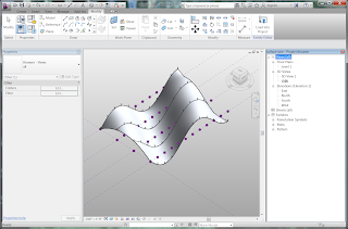
Click each model line of the line sine objects. You may have to hover and tab to select the model line and not the entire instance. Use Create Form to produce a smooth surface.

Play with the phase, amplitude, and frequency to make new surfaces. You can also change the spacing of the grid. The forms can be very complex.

To model a different curve, simply change the formula in the point family. You can look up formulae on the Web. For example, a catenary curve equation is found at
http://classroom.synonym.com/calculate-catenary-2651.html
  • y = a/2 (e^(x/a) + e^(-x/a)) 
where e is the base of the natural logarithm and is approximately 2.71828.

Sunday, September 1, 2013

Palladian architecture with Revit constraint modeling

The designs of Palladio have had an important influence on architecture for over four hundred years.


The Villa Rotunda in Vicenza is a masterpiece of Renaissance and Neo-Classical architecture. 


Palladian design came to America and influenced architecture throughout the colonies and the states. 

The southern plantation houses of my native state of Louisiana were inspired by Palladio. It is interesting to study them as a house type. 

In Chalmette, the Beauregard House is one masterpiece.This house near New Orleans is part of a National Historic Park and is open to the public. It is a prototypical design for a plantation house (although not actually associated with a plantation.)


Oak Alley, on the banks of the Mississippi River north of New Orleans is another masterpiece.


Destrehan is another example, older than the other two and not as refined.


A plantation house is a good exercise in the use of constraints to enforce symmetry and proportion.


The first step in a project done with Revit is much like the first step in a project done on paper. Draw the site, using the Massing & Site -> Toposurface tool. Draw a Property Line using the same menu. From the Manage->Project Information, you can describe the client, the location, and, using the Energy Settings parameter, choose a Location Weather and Site value.


For most buildings, the architect knows very early in the process how many stories there are, although the exact height of each story may not be known. Switch to an Elevation view and then use the Home->Level command to draw a Level 1 and Level 2. You can rename the levels and set the heights of the levels after you draw them.


Most real buildings are based on a grid that helps define the structure. A Palladian villa or Louisiana Plantation House typically has a symmetry that is defined by a grid. From a Plan view, use the Home->Grid command to draw lines for the grid.


Symmetry is based on the establishment of centerlines. If you pick the centerline, you will see a dimension line. You can click on the little icon of a dimension line to make the "temporary dimension" into a "permanent dimension. Then, you can set the grid line to have neighboring grid lines that are equally spaced.


You can also draw an aligned dimension line with to locate several reference grid lines, and then set them to be equally spaced by clicking on the EQ icon.


To make the drawing look tidy, you can drag the dimension lines until the leaders and lines are all aligned.


Having draw the grid lines and dimensioned them to control the bay proportions, you can easily draw walls. It is actually best to draw the walls away from the grid lines. Once you have drawn the walls, you can drag them to the dimension line. A lock icon should appear, and you can lock wall to the grid.


 This just shows more locking of walls, this time on the Level 1. Notice in the Properties box to the left that the Top Constraint is set to "Up to level: Level 2". The walls on the Ground floor should have a Top Constraint of "Up to level: Level 1". This command sets the height of the wall to the level. If you later change the level in a section or elevation view, the wall will remain constrained to the level above.
This just shows more locking of walls, this time on the Level 1. Notice in the Properties box to the left that the Top Constraint is set to "Up to level: Level 2". The walls on the Ground floor should have a Top Constraint of "Up to level: Level 1". This command sets the height of the wall to the level. If you later change the level in a section or elevation view, the wall will remain constrained to the level above.


Here a roof is being drawn, but the roof has a "Base Level" of Level 1. It should be Level 2. You can change the parameter and the roof will jump up to the right location.


A second roof can be drawn to provide the double pitch that is characteristic of Louisiana plantation. 
From the View menu, one can draw a section cut line in a plan view. This does not merely draw the symbol for a section cut, but generates the entire section too.

If you want the section to have walls and floors as a solid fill, you can easily change the View Properties by using the Visibility/Graphics Overrides parameter. Set whichever objects are needed to have a solid fill.


Draw the interior walls on each level. It is easiest to sort of sketch them in, deliberately avoiding the grid lines. Once they are drawn and trimmed properly, you can drag them to the grid line and then lock them in place to align with the grid line.


On another level, the process is repeated to lock the walls to the grid lines.


The French windows are drawn using a door family. First you must load the Door family from the library. The family defines the basic un-dimensioned form of a French window. You will add the dimensions later.


Once the door is loaded, you use the button for Edit Type to define a new door type that you can insert repeatedly. Duplicate the current type and give it an appropriate name.


Having duplicated the type, you can edit the Dimensions, such as the width and height.


You can insert the doors into the walls. Again, the best way is to place them imprecisely. You can then drag them to the right location and use the EQ icon to center them between walls.


If necessary, use the Aligned linear dimension to set the dimensions to be equal.


An entablature can be added with the Beam tool. You can load a timber family and then establish the dimensions of the beam by Edit Type.


From the 3D view, you can see the beam along the outside edge of the roof.


You can edit the "sketch" of the beam to get it aligned with the appropriate part of the roof.


There is a Doric column family in the standard library. Load the family and then add columns around the outside edge. You can use dimensions to lock the columns a distance from the grid lines and align them to grids as centerlines.


Here the dimension is being used to set the end column away from the grid line by 1'2".


The columns by default have a top attachment to the Level 1. You can change the Top Level to the Level 2 and they will stretch to a double height.


The columns also have a Top Offset of -1'4" which places them at the bottom of the beam that represents the entablature. Once you get one right, you can copy them around the building.Or, if you have already placed them, select them all and change their parameters at once. 


This is a good time to "flex" the model by moving the grid lines and levels around. If you have properly locked everything to the lines, the house will reshape. 


The doors seem too short. You can create a new type of door and quickly change all of the doors to the new type.


As you can see, the elements are heavily constrained to the grid lines.


A porch floor was inserted and shadows were turned on. Now the model can be changed in proportion by simply moving the grid lines.


The basic form of the type is complete and fully constrained. Stairs, railings, chimneys, and other elements can be added and locked to appropriate lines. 

Alternative columns could be modeled and quickly substituted. Different door and window families could be collected to allow rapid substitution.

The implications of using constraints and locks to hold a model into a set of relationships is that one can model a building type and then rapidly make instances of the type. The rich formal systems of sameness and variation that make American traditional cities so beautiful can be expressed with BIM tools.